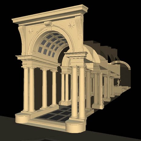
Rendering of the Gallery (E. Garbin, LAR, DPA, IUAV)
Rendering of the Gallery (E. Garbin, LAR, DPA, IUAV)
The
Borromini Gallery in Palazzo Spada, Rome
Ideal regular model and
deformed real model
Abacus
of the perspective deformations
Camillo Trevisan
trevisan@iuav.it
Paper in PDF format (980
kB) ![]()
Versione italiana
Programme of the conference held May 19th 1999
Centro Svizzero di Cultura di Roma
part of the cycle "Prospettiva e Prospettive"
edited by prof. Rocco Sinisgalli
September 1999
Best view 1280x1024
Any
attentive observer visiting and walking through the Gallery of Palazzo Spada, in
Rome, will be struck by a real and deliberate contradiction: he witnesses a
deformed architectural structure but perceives – due to rational
decodification – an ideal regular gallery in which the columns are all of the
same height and equidistant from one another.
In reality, a similar experience occurs every time we observe a perspective or a
photograph. Nevertheless, in this case the scenic effect created by entering
into a perspective, enabling us to run it through in its entirety even to an
uncertain and unfamiliar threshold, projects us into a new dimension. This
resulting light dizziness is then accentuated by the continuous modification of
both what we can see and what we perceive. Once this immediate visual wonder has
been overcome, the desire to understand remains. How was the Gallery created?
Which rules does it follow? How should it be followed if we want to recreate the
evident correspondence with a regular gallery? And with which regular gallery?
The aim of this study is to present the answers to some of these questions.
The first section investigates and studies in detail the configuration of the
real gallery, suggesting the existence of a method which is not perspective of
the arrangement in depth of the columns and the floor panels.
Since the disposition of the columns does not follow a perspective – and there
is therefore no projective mechanism which places the Gallery in a close and
biunique relationship to a family of regular models – it is justified to ask
if a regular interpolating model exists, preferable to all the other, infinite,
possible regular models. The second section studies the ideal regular model
under the guidance of proportional research in the absence of indications of a
distinctively projective type. Finally, the last section examines in detail the
geometrical analysis, subdividing and illustrating the effects of the variations
of some constructive parameters of a solid perspective.
The appendix includes some methods of geometrical construction of a solid
perspective, illustrating the use of a software for the generation of
solid perspectives and their counter deformation. Finally, it includes the
definitions of the nomenclature used in the article.
1.
The characteristics of the arrangement of the columns and panels of the floor in
the real Gallery
Rocco Sinisgalli [1]
has pointed out, after careful research, that the Gallery in Palazzo Spada is
not really a true and characteristic solid perspective. Or rather, of the two
fundamental characteristics of a solid perspective – but also of a linear
perspective, that is the convergence of orthogonals of the projection plane
towards a single vanishing point and the arrangement in depth of the objects in
function of their distance from the viewpoint – only the former is rigorously
respected and verified. In fact, if a single vanishing point [2]
exists, nevertheless the vertical axis of the 12 pairs of columns of the real
Gallery are not placed planimetrically following a rigorous perspective
arrangement [3] (cf. figure 1.1 and 1.2).
A generic regular model [4],
deformed in solid perspective so that its first and last columns coincide with
the first and last column of the real Gallery, does therefore not maintain the
coincidence of the other intermediate columns too with the same of the solid
perspective: the greater the distance at the beginning or end of the Gallery,
the greater their displacement will be with respect to the foreseen position in
a true solid perspective.[5]
In other words, although they do not refer to the scheme of deformation of a
regular model scanned by identical intercolumns, the columns of the Gallery
Spada do not refer to the scheme of deformation of a regular model (cf. fig.
1.2). The attempt to answer the following question is therefore of great
interest: why did Borromini choose precisely that arrangement in depth instead
of that perspective? Does a clear and connecting rule exist between the
planimetrical positions of the axis of the columns or were they positioned
following inscrutable and indefinable subjective mechanisms, simply liberally
modifying a basic perspective arrangement?
An accurate analysis of the data of the measurements of the inter-axis and of
the original floor panels leads us to the conclusion that a rule does exist and
it is defined by a geometrical series.
Let us assume, in fact, that the series begins with a seed of five roman
palms (60 ounces). The distance between the axis of the first two columns will
thus be equivalent to 60 ounces and the length of the first floor panel,
including the first space, equivalent to 12 ounces, a fifth of sixty). To define
the successive inter-axis (and the successive panel), a reduction of the
proportion 5/6 is adopted; the second inter-axis (and panel) will therefore be
50 ounces (10 ounces for the second space, a fifth of fifty). The third length
of the series will be equivalent to five sixths of fifty, that means 41 ounces
and two thirds.
From the fourth element of the series being constructed the coefficient of
reduction changes, going from 5/6 (10/12) to 11/12 and from 1/5 to 1/4 for the
space between panels. The fourth length of the series will therefore be
equivalent to eleven twelfths of 41 and 2/3 and so on to the last inter-axis and
the last floor panel.
Even though it has nothing to do with the perspective, this form of detailed
arrangement in depth produces a sequence that is much more modulated, without
any effect of muddle of the columns towards the end of the Gallery and reducing
the length of the first lacuna (cf. fig. 1.1).
Before discussing this hypothesis very closely, two preliminary considerations
are necessary.
The first concerns the transformation in roman palms of the measurements taken
in metres. Not only do different measurements exist in reference to the palm [6],
but also the instruments themselves, which are used, could be slightly
different, depending on the reference sample. Furthermore, ignoring minor errors
of construction and survey, it is therefore not possible to define the length of
the Gallery or its width of the various inter-axis in palms with absolute
precision. To complicate the problem further, the columns are deformed and
slightly off axis with respect to the plinths.[7]
There is another aspect to be considered – although the successive reductions
(5/6, 5/6, 11/12, 11/12, 11/12, etc.) produce rational numbers, which can be
easily expressed as fractions amongst small wholes, they soon produce fractional
values, which are difficult to identify. For example, the last value of the
series is equivalent to 434.00218599… ounces. We therefore round off to the
nearest ounce, or to the fifth of an ounce (a minute). In the latter case one
obtains better results than rounding off to the ounce (cf. table 1 and 2, column
4 and 7); however, considering that a minute is less than 4 millimeters, it
seems excessive, if not impossible, to think that so much extra calculation was
carried out.
To verify the hypothesis, a computer program has been developed. It is able to
reduce the mean least square between the data produced by the proposed
geometrical series and those measured, also modifying the coefficient of
transformation from meters to palms apart from a translation factor which moves
the grid calculated with respect to the one measured together, to reduce the
difference. As can be seen upon close examination of tables 1 and 2 and figure
1.3, the variation of the rounding off modifies only minimally both the mean
least square and the conversion coefficients (the final models differ by not
more than 1.8 mm); basing the first around a centimeter, the second on the
values of 0,22445 for the calculation of the inter-axis and of 0.22285 for the
floor panels.[8]
There is therefore a difference of around a millimeter and a half between the
measurements of the two roman palm samples; this data could lead us to believe
the technicians who placed the columns and those who constructed the floor used
different instruments.
The theoretical distance between the first and last axis is therefore equivalent
to 434 ounces (36 palms and 1/6); even if the same tables show that the first
inter-axis seems to have been moved back by one ounce, ideally bringing the sum
of the inter-axis to 435 ounces (36 palms and 1/4) and that of the panels to 430
ounces (35 palms and 5/6).
This scheme is therefore very close to the real Gallery with respect to a solid
canonical perspective, which differs from the Gallery with average and maximum
deviations, which are five times greater.
Finally, it should be noted that geometrical series, which are completely
analogue to those proposals, can also be obtain via graphics and with great ease
and proportional accuracy (cf. figure 1.4).[9]
If this was the method used to position the columns and the floor panels, it
naturally leads to the use of the 12 viewpoints to deform them, one column at a
time.[10]
Indeed, once the positions of the axis were found, it was necessary in each case
to deform each column perspectively both on the plane and in height. A
combination of the two mechanisms which have been illustrated is always valid
for the deformation: the convergence of the orthogonals to the frontal plane
towards the common vanishing point and the reduction in depth, this time not of
the inter-axis but of the plinths, of the bases, of the shafts and the capitals
of the columns.
The adoption of a centre
of deformation for each column – placed in a sequence that reproduces the
arrangement in depth from the axis – means that the deformation is contained
within acceptable limits from the viewpoint of an observer walking along the
Gallery.
Thus,
the Gallery seems to have been built on the basis of separation and accumulation
of the effects derived from different mechanisms: the perspective pyramid that
converges to the vanishing point; the geometrical arrangement in depth of the
principal elements; the individual deformation, once again perspectively, of
each column of the Gallery.
Figure 1.1 Comparison of the plane of the real Gallery (in red) and the regular deformed model with perspective method (in blue), so as to make the axis of the first and last columns coincide with the same columns of the real Gallery. To the left the deviations between the axes are highlighted, in meters. To the right, the deviations between the floor panels. The mean least square for the axis is equivalent to 8 centimeters; for the floor panels it is 10 centimeters.
Figure 1.2 To the left, the comparison of the ideal regular model (in blue) and the counter deformation of the real Gallery (in red). To the right, the verification of the presence of more than one viewpoint and dimensions of the ideal regular model (cf. section 2), expressed in roman palms.
Figure 1.3 Comparison of the plan of the real Gallery (in red) and the arrangement in depth generated by the geometrical series illustrated in section 1. To the left the deviations between the axes can be seen in centimeters. To the right, the deviations of the floor panels. Mean least square is approximately 1 centimeter, both for the axis and for the floor panels.
Figure
1.4
Graphic method
for the construction of the geometrical series of reduction. Once the segments
are defined – AB (60 ounces, first inter-axis), BC (26.666 ounces), BD (40
ounces), BE (45 ounces) and BF (53.333 ounces), pointing the compass on A with
opening AB, trace the first arc to cross the segment AD. By lowering the
perpendicular to AB, the length of the second inter-axis is defined and so on.
The line AD corresponds to a reduction equivalent to 0.8321 (5/6 = 0.8333,
difference of 0.0012); the line AC to 0.9138 (11/12 = 0.91666, difference of
0.0029; AE to 0.8 (4/5 = 0.8) and finally, AF to 0.7474 (3/4 = 0.75, difference
of 0.0026).
Figures A. 1-3
Graphic
method of construction of solid perspective (cf. appendix A).
Table 1 – Column inter-axes (cf. figure 1.3)
| 1 m | 2 ounce | 3 o | 4 cm | 5 ounce | 6 ounce | 7 cm | 8 ounce | 9 ounce | 10 cm | |||
|
1 |
0.0000 |
0.00 |
0 |
-1.2 |
0.00 |
0.0 |
-1.3 |
0.00 |
0.00 |
-1.2 |
||
|
2 |
1.1447 |
61.20 |
60 |
1.0 |
61.19 |
60.0 |
0.9 |
61.19 |
60.00 |
1.0 |
||
|
3 |
2.0958 |
112.06 |
110 |
2.6 |
112.03 |
110.0 |
2.5 |
112.03 |
110.00 |
2.6 |
||
|
4 |
152 |
151.6 |
151.67 |
|||||||||
|
5 |
3.5400 |
189.28 |
190 |
-2.6 |
189.24 |
189.8 |
-2.3 |
189.23 |
189.86 |
-2.4 |
||
|
6 |
4.2159 |
225.41 |
225 |
-0.5 |
225.37 |
224.8 |
-0.2 |
225.36 |
224.87 |
-0.3 |
||
|
7 |
4.8271 |
258.09 |
257 |
0.8 |
258.04 |
256.8 |
1.0 |
258.04 |
256.97 |
0.8 |
||
|
8 |
286 |
286.2 |
286.39 |
|||||||||
|
9 |
5.8653 |
313.60 |
313 |
-0.1 |
313.54 |
313.2 |
-0.6 |
313.53 |
313.35 |
-0.9 |
||
|
10 |
6.3336 |
338.64 |
338 |
0.0 |
338.57 |
338.0 |
-0.2 |
338.56 |
338.07 |
-0.3 |
||
|
11 |
6.7545 |
361.14 |
361 |
-1.0 |
361.07 |
360.8 |
-0.8 |
361.06 |
360.73 |
-0.6 |
||
|
12 |
382 |
381.6 |
381.51 |
|||||||||
|
13 |
7.4993 |
400.97 |
401 |
-1.3 |
400.89 |
400.6 |
-0.7 |
400.88 |
400.55 |
-0.6 |
||
|
14 |
7.8390 |
419.13 |
418 |
0.9 |
419.05 |
418.0 |
0.7 |
419.04 |
418.00 |
0.7 |
||
|
15 |
8.1419 |
435.33 |
434 |
1.3 |
435.24 |
434.0 |
1.0 |
435.23 |
434.00 |
1.1 |
||
| MLS in centimeters |
1.3 |
1.2 |
1.2 |
|||||||||
| Translations in ounces |
0.65 |
0.69 |
0.65 |
|||||||||
| Conversion meter/palm |
0.224434 |
0.22448 |
0.224485 |
|||||||||
Table 2 – Floor panels (cf. figure 1.3)
| 1 m | 2 ounce | 3 o | 4 cm | 5 ounce | 6 ounce | 7 cm | 8 ounce | 9 ounce | 10 cm | |
|
1 |
0.0000 |
0.00 |
0 |
-2.7 |
0.00 |
0.0 |
-3.0 |
0.00 |
0.00 |
-2.8 |
|
2 |
0.9178 |
49.42 |
48 |
-0.1 |
49.42 |
48.0 |
-0.3 |
49.41 |
48.00 |
-0.2 |
|
3 |
1.1308 |
60.89 |
60 |
-1.1 |
60.89 |
60.0 |
-1.3 |
60.88 |
60.00 |
-1.2 |
|
4 |
1.8455 |
99.38 |
98 |
-0.2 |
99.37 |
97.6 |
0.3 |
99.36 |
97.50 |
0.6 |
|
5 |
2.0525 |
110.53 |
110 |
-1.7 |
110.52 |
110.0 |
-2.0 |
110.51 |
110.00 |
-1.9 |
|
6 |
2.6538 |
142.90 |
142 |
-1.0 |
142.90 |
141.2 |
0.2 |
142.88 |
141.25 |
0.2 |
|
7 |
2.8349 |
152.66 |
152 |
-1.5 |
152.65 |
151.6 |
-1.0 |
152.64 |
151.67 |
-1.0 |
|
8 |
3.3794 |
181.98 |
180 |
1.0 |
181.97 |
180.2 |
0.3 |
181.95 |
180.31 |
0.2 |
|
9 |
3.5546 |
191.41 |
190 |
-0.1 |
191.40 |
189.8 |
0.0 |
191.39 |
189.86 |
0.0 |
|
10 |
4.0592 |
218.59 |
216 |
2.1 |
218.58 |
216.0 |
1.8 |
218.56 |
216.12 |
1.7 |
|
11 |
4.2135 |
226.90 |
225 |
0.8 |
226.89 |
224.8 |
0.9 |
226.87 |
224.87 |
0.9 |
|
12 |
4.6675 |
251.34 |
249 |
1.6 |
251.33 |
248.8 |
1.7 |
251.31 |
248.94 |
1.6 |
|
13 |
4.8168 |
259.38 |
257 |
1.7 |
259.37 |
256.8 |
1.8 |
259.34 |
256.97 |
1.6 |
|
14 |
5.2159 |
280.88 |
279 |
0.8 |
280.86 |
278.8 |
0.9 |
280.84 |
279.03 |
0.5 |
|
15 |
5.3553 |
288.38 |
286 |
1.7 |
288.36 |
286.2 |
1.1 |
288.34 |
286.39 |
0.8 |
|
16 |
5.7186 |
307.95 |
306 |
0.9 |
307.93 |
306.4 |
-0.1 |
307.90 |
306.61 |
-0.4 |
|
17 |
5.8530 |
315.18 |
313 |
1.3 |
315.16 |
313.2 |
0.7 |
315.14 |
313.35 |
0.5 |
|
18 |
6.1864 |
333.14 |
332 |
-0.6 |
333.12 |
331.8 |
-0.5 |
333.09 |
331.89 |
-0.6 |
|
19 |
6.3108 |
339.84 |
338 |
0.7 |
339.82 |
338.0 |
0.4 |
339.79 |
338.07 |
0.4 |
|
20 |
6.6135 |
356.13 |
355 |
-0.6 |
356.11 |
355.2 |
-1.3 |
356.08 |
355.07 |
-0.9 |
|
21 |
6.7299 |
362.41 |
361 |
-0.1 |
362.38 |
360.8 |
0.0 |
362.35 |
360.73 |
0.2 |
|
22 |
6.9987 |
376.88 |
377 |
-2.9 |
376.86 |
376.4 |
-2.1 |
376.82 |
376.31 |
-1.9 |
|
23 |
7.1082 |
382.78 |
382 |
-1.3 |
382.75 |
381.6 |
-0.8 |
382.72 |
381.51 |
-0.6 |
|
24 |
7.3720 |
396.98 |
396 |
-0.9 |
396.96 |
395.8 |
-0.8 |
396.92 |
395.79 |
-0.7 |
|
25 |
7.4715 |
402.34 |
401 |
-0.2 |
402.32 |
400.6 |
0.2 |
402.28 |
400.55 |
0.4 |
|
26 |
7.7054 |
414.94 |
414 |
-1.0 |
414.91 |
413.6 |
-0.5 |
414.88 |
413.64 |
-0.5 |
|
27 |
7.7950 |
419.76 |
418 |
0.6 |
419.74 |
418.0 |
0.3 |
419.70 |
418.00 |
0.3 |
|
28 |
8.0090 |
431.28 |
429 |
1.5 |
431.26 |
429.0 |
1.2 |
431.22 |
429.00 |
1.3 |
| MLS in centimeters |
1.2 |
1.0 |
0.9 |
|||||||
| Translations in ounces |
1.46 |
1.59 |
1.52 |
|||||||
| Conversion meter/palm |
0.22284 |
0.22285 |
0.222875 |
|||||||
Explanation of tables 1 and 2 (cf. figure 1.3)
Column
1
Here we find the measurements
calculated on the inclined plane of the Gallery and projected on the horizontal
plane (cf. Rocco Sinisgalli, Una storia della scena prospettica …, op.
cit., p.17). To facilitate the reading and comparison of the data, the first
value of each table is zero. In the first table the positions of the axis of the
columns measured are noted (the intersecting points of the diagonals of the
quadrilaterals of the bases are considered axis of the columns, even if other
reference points could have been considered; see, for example, the first columns
with the torus that protrudes from the base). On the other hand, in the second
table we have a list of the initial and final positions of the fourteen original
floor panels. Unit of measurement: meter.
It should be noted in table 1 that rows 4, 8, 12 correspond to the lacuna
placed between the four groups of three columns: for this reason there are no
data since there are no columns in those positions. However, the geometrical
series does include the lacunas (columns 3, 6, 9 of table 1).
Columns 2, 5,
8
In these columns we can see the
equivalent measurements in meters of the first column of the table in ounces.
Since the precise characteristics of the instruments used to construct the
Gallery are not known, various hypothesis have been formed (cf. columns 3, 6,
9), each of which shows a slightly different result in function of the
coefficient of conversion between the meter and the roman palm.
Columns 3, 6,
9
To verify the hypothesis of the
geometrical series (with reference to the disposition of the axis of the columns
and the floor panels), above all, it is necessary to convert the measurements
from meters to roman palms or rather to ounces (1 palm = 12 ounces). The
hypothesis foresees a starting point (both for the first inter-axis and for the
first floor panel, equivalent to 60 ounces (5 palms) and a progressive reduction
of the intervals, equivalent to 5/6 for the first two successive intervals and
to 11/12 for all the others (the spaces between the floor panels are easily 1/5
the size of the interval in the first two cases and 1/4 in all the others). The
sequence of reduction produces, however, values which have not always been
rounded off (cf. column 9). However, other two hypotheses are considered: the
first foresees the rounding off to the ounce (column 3), the second to a fifth
of an ounce (the minute). Such hypothesis considers the coefficients of
conversion from meter to palm slightly differently to let the proposed
hypothesis coincide more accurately with the hypothesis proposed with the
calculation. However, the difference is minimal.
Columns 4, 7,
10
Deviations expressed in centimeters between the hypothesis and calculated values and converted to ounces (cf.
columns 2, 5, 8).
Therefore, the columns 2, 3, 4 refer to the hypothesis of rounding off to the
ounce of the value calculated for the geometrical series; columns 5, 6 and 7 to
the rounding off to a fifth of an ounce; columns 8, 9, 10 to the values which
have not been rounded off. The hypothesis regarding columns 2, 3, 4 seems more
likely for both tables even if it is not the best result of the deviations.
In figure 1.3 the deviations are illustrated in 2 tables (column 4) between the
axis and the real and calculated floor panels.
The
mean least square (MLS) is expressed in centimeters and indicates the “quality”
of interpolation with a single statistical value. In fact, in this data, the
major deviations “weigh” more heavily than the others, since the deviations
themselves are squared.
The translation, in ounces, shows the displacement of the data together shown in
columns 3, 6, 9 to reduce the deviation between this data and the data present
in columns 2, 5, 8 to a minimum. The translation corresponds to the deviation of
the first values of columns 4, 7, 10 (expressed here in centimeters).
The values of conversion from meters to roman palms (all different but taken
with a close approximation around the average value of 0.224 meters per palm),
take the values calculated in columns 2, 5, 8 into account. The slight
differences between the values found may be explained – apart from their
constructive imprecision – also by the different instruments used by the
builders.
Finally, it should be noted that, as has already been said, the calculated
measurements were projected on a horizontal plane with a reduction equivalent to
0.99556 (a cosine of 5.4° inclination of the floor of the Gallery). If the
measurements of the geometrical series found had been used directly on the
inclined plane – as seems probable – the values of conversion from meters to
roman palms would undergo a slight increase (1.00446), rising respectively to
0.2255 (for the axis, table 1) and 0.2255 (for the floor panels, table 2);
keeping the values presented in both tables unchanged and taking into
consideration all things said so far.
2.
The regular models and the ideal regular model: dimensions
and proportions from a constructive point of view
Even though it has
been verified that there is no regular model at the basis of the real Gallery
(cf. figure 1.1 and section 1), even if there may be an infinite number of
regular models, which, once deformed, interpolate the Gallery itself, it is
still evident that the architect needs to consider an ideal regular model as
reference. The definition of the arrangement in depth of the columns and of the
floor panels is not at all sufficient for the completion of the project: for
example, how many paneled ceilings should be taken into consideration each
time? What proportions should be given to the columns, to the trabeation and to
the bases? Which regular inter-column should be adopted? To be able to answer
these and other questions it is necessary to consider the measurements of the
calculation (in roman palms):
|
|
palms |
fractions |
modules |
|
Diameter of first column at base (module) |
1 |
2/3 |
1 |
|
Distance in breadth between columns (internal face of frontal first couple) |
14 |
- |
8.4 |
|
Distance between axis of 2 internal frontal columns |
15 |
2/3 |
9.4 |
|
Distance between axis of 2 external frontal columns |
20 |
1/3 |
12.2 |
|
Distance in breadth between bases |
13 |
- |
7.8 |
|
Distance in breadth between axis of first two pairs of columns |
2 |
1/3 |
1.4 |
|
Total height of columns (with base, capital excluding plinth and abacus) |
13 |
1/3 |
8 |
|
Diameter of facade arch |
13 |
1/3 |
8 |
|
Total height of trabeation |
3 |
- |
1.8 |
As
has already been noted, when looking at the front of the colonnade, there are an
infinite number of regular models – that is, an infinite possibility of
inter-columns – that satisfies the question: finding an ideal model in which
the axis of the first and last columns are superimposed upon the axis of the
first and last column of the real calculated model. Using the measurements of
the paneled ceilings placed on the vault, it is, however, possible to define a
regular model - that fulfils the requirement of maintaining the paneled ceilings themselves squares - better than the others. Accordingly, the
paneled ceilings of the vault are the only useful evidence in defining the dimensions of
the regular model which we would define “ideal”.
To define the inter-columns of such a model, the paneled ceilings are to be
considered as squares.
The arch contains seven paneled ceilings (width 8 intervals), placed in rays
with an additional belt on the right and left of the base of the arch itself.
Since the diameter of the arch facade is equivalent to 13 1/3 palms, its
development corresponds to approximately 21 palms. Taking into consideration
that the two belts at the impost of the arch have a width of 1.2 palms each,
18.6 palms remain. Thus, if one paneled ceiling is 2.6 palms: 2.2 p. + 0.4 p.
of space – we get 2.2 x 7 + 0.4 x 8 = 18.6 palms.
In depth the arcades contain four paneled ceilings with three intervals,
equivalent to two inter-columns plus a module (a diameter of a column). Thus,
two inter-columns plus a module are equivalent to: 2.2 x 4 + 0.4 x 3 = 10 palms
(6 modules).
Therefore, the inter-column is equivalent to 4 1/6 palms (2 1/2 modules: the
elegant and solid Eustilo), whereas the inter-axis is equivalent to 3.5 modules
= 5 5/6 p. With these measurements, the paneled ceilings turn out to be squares
and the overall dimensions sufficiently “round”, with a total height of the
columns corresponding to the diameter of the arch facade (8 modules) and to the
length of the three groups of columns (2.5 x 2 + 3), measured on the external
surface of the three columns.
Each group of three columns therefore contains a perfect cube.
In short, the proposed hypothesis produces the following ulterior measurements
(cf. figure 1.2):
|
|
palms |
fractions |
modules |
|
Length of ideal colonnade [11] |
84 |
1/3 |
50.6 |
|
Inter-axis of columns |
5 |
5/6 |
3.5 |
|
Length of floor panels (with space) |
5 |
5/6 |
3.5 |
|
Space between panels (equal length/depth) |
1 |
- |
0.6 |
|
Breadth of floor panels |
3 |
- |
1.8 |
|
Length of bases (3 columns) |
14 |
1/3 |
8.6 |
|
Distance between bases (lacuna) |
9 |
- |
5.4 |
|
Distance between axis of two final internal columns |
11 |
- |
6.6 |
|
Distance between column plinths |
3 |
1/2 |
2.1 |
|
Length and depth of column plinths |
2 |
1/3 |
1.4 |
|
Breadth of base (one column) |
2 |
2/3 |
1.6 |
|
Breadth of base (two columns) |
5 |
- |
3 |
This
“ideal” model can be “projected” to define a solid perspective so that
the axis of the first and last column are superimposed on the axis of the first
and last column of the real Gallery (cf. figures 1.1 and 1.2).
The parameters of transformation are:
Plane of the traces:
placed on the axis of the first column
Viewpoint:
distance from plane of traces is 5 2/3 palms; height: 6 2/3 palms
(approx. 1.5 meters)[12]
Vanishing point:
distance from the plane of traces is 69 2/3 palms.
3. Study of the mechanism of
perspective deformation: definition of the limits, the extreme results and
implications and links that exist between visual construction and fruition
The observations
that follow refer to a construction of the solid perspective corrected from a
geometrical point of view: without, therefore, the proportional alterations,
which are characteristic of the Gallery in Palazzo Spada (cf. section 1).
The main objective of these examples is to highlight the role of each parameter
of visual construction and fruition: the viewpoints and vanishing points, the
plane of traces and the eye of the observer.[13]
Indeed, it is not only the choice of constructive parameters that greatly
influences the deformed model – very often difficult to understand and
classify even if geometrically inevitable – but the same visual fruition of
the solid perspective follows a logic which apparently seems unexplainable.
Two series of examples have therefore been chosen: the first – paragraphs
3.1.1-5 – analyses the modifications undertaken in the solid perspective in
the variation of one or more constructive parameters (the viewpoint, the
vanishing point or the plane of the traces); the second – paragraphs 3.2.1-3
– studies the phase of ideal reconstruction of the regular model varying the
position of the eye of the observer who explores the solid perspective.
Moving along the solid perspective, for example, the height of the observer with
respect to the floor remains constant. Walking along the inside of a solid
perspective at a constant speed therefore corresponds to – in the interior of
an ideal regular model – a displacement also in height and with an accelerated
or decelerated movement, according to the direction.
If both are observed from the viewpoint used for the construction of the solid
perspective the initial regular model and the solid perspective coincide.
This superimposition is maintained even when the perspective plane is rotated
and inclined: the two models remain superimposed – in perspective –
precisely because the lines that join each point of the regular model with the
viewpoint also pass along the same points of the solid perspective, regardless
of the position of the perspective plane.
Since all the semi lines which irradiate from the viewpoint and pass along any
point of the solid perspective, also pass along the same point of the regular
model, the observer, with his eye on the constructive viewpoint need not,
however, necessarily direct his eye towards the vanishing point.
In other words, if we place the focus of the lens of a camera on the
constructive viewpoint, in the photograph the solid perspective and the initial
regular model are superimposed regardless of the rotation of the lens.
3.1 Modification of the solid perspective to
vary the parameters (the regular model remains constant)
In the
first five examples the regular model is kept constant whereas the constructive
parameters (the viewpoint and vanishing point and plane of the traces) are
either varied one at a time or in pairs. The resulting solid perspective will
therefore have characteristics, which will closely depend on the variations. The
derived characteristics can be combined amongst each other generating infinite
possibilities of overall variations.
3.1.1
Variation of the solid perspective with displacement of the viewpoint (cf.
figure 3.1.1)
If the regular model, the vanishing point and the plane of the
traces are kept constant, the displacement of the viewpoint along the
axis of symmetry, the solid perspective is deformed. Such a model will
constrict in length if the viewpoint moves away from the vanishing point;
it will expand – towards the vanishing point - if
the opposite is the case.
3.1.2 Variation of
the solid perspective by displacing the vanishing point (cf.
figure 3.1.2)
Keeping the regular model, the viewpoint and the plane of the
traces constant, the displacement of the vanishing point along the
axis of symmetry deforms the solid perspective. Such a model will
decrease in length if the vanishing point moves towards the viewpoint;
it will increase – towards the vanishing point – if the opposite is
the case.
3.1.3
Variations of the solid perspective by displacing the plane of the
traces (cf.
figure 3.1.3)
Keeping the regular model, the vanishing point and the viewpoint
constant, the displacement of the plane of the traces along the axis
of symmetry deforms the solid perspective. Such a model will increase if
the plane of the traces moves away from the viewpoint; it will
decrease – towards the vanishing point – if the opposite is the case.
3.1.4 Variations
of the solid perspective by displacing both the vanishing point and
the plane of the traces (cf.
figure 3.1.4)
Keeping both the regular model and the viewpoint constant, the
displacement of both the vanishing point and the plane of the traces together
will modify the scale of the solid perspective. Such a model will be
enlarged – maintaining the proportions of its parts – if the vanishing
point and the plane of the traces move away from the viewpoint;
it will be reduced – towards the vanishing point – if the opposite is
true.
3.1.5
Variations of the solid perspective by displacing the viewpoint
and the vanishing point with respect to the axis of the regular model (cf. figure 3.1.5)
If the viewpoint
and the vanishing point define a line, which does not belong to the
vertical plane of symmetry of the regular model, the resulting solid
perspective will not keep its right-left symmetry but will generate an “oblique”
model. However, by varying the height of the viewpoint with respect to
the vanishing point (placed on the symmetrical plane of the regular
model), the solid perspective will obviously maintain its right-left
symmetry: the only differences regard the height.
3.2 Modifications of the
regular model varying the parameters (constant solid perspective)
In these examples
the solid perspective remains constant while the observer places his eye in
different positions to the point used to construct the solid perspective itself.
He will therefore see – from a geometrical point of view – a regular model
which differs from the initial one (it would be identical only if the observer’s
eye were placed on the constructive viewpoint). Some “regularities” were
maintained – such as the arrangement in depth of the inter-axis. Others,
however, were changed.
3.2.1
Variation of the regular model by the movement of the observer’s eye
along the line for the viewpoint and the vanishing point (cf. figure 3.2.1)
By placing the eye
in any other position of the line for the viewpoint and the vanishing
point other than the viewpoint, the solid perspective and the regular
model do not coincide. Nevertheless, for each point of observation along the
line, there is a regular model – different to the original – and it
too is regular: the only difference between these infinite regular models
and the original regular model is due to a compression along the axis and
therefore, in this example, due to the diverse inter-axis of the columns. If the
eye moves closer to the vanishing point, the inter-axis becomes
smaller; it expands, however, if the eye moves away from the vanishing point.
3.2.2
Variation of the regular model by the movement of the eye of the
observer above or below the line for the viewpoint and the vanishing
point (cf. figure 3.2.2)
If the eye is raised
or lowered with respect to the viewpoint, the regular model is no
longer completely regular: in fact, the floor is inclined towards the top or the
bottom. It should be noted that the columns of the “regular model” restored
in this manner still remain parallel to one another and are all of the same
height: the observer who places his eye higher with respect to the viewpoint will
still see a descending ramp which is regular; if the eye is lowered, the
ramp will be ascending, but still regular.
3.2.3
Variation of the regular model by moving the eye of the observer
to the right or to the left of the line for the viewpoint and vanishing
point (cf.
figure 3.2.3)
If the eye moves to the right or left with respect to the viewpoint, how
does the regular model change? In this case the Gallery becomes oblique
but the colonnades still remain parallel to one another. It is evident that the
effects can add up: if the observer moves the eye further forward, above and,
for example, to the left with respect to the viewpoint, he will see a
regular gallery restored with the inter-axis of the columns compressed with
respect to the standard regular model (eye moved further forward
with respect to the viewpoint). Furthermore, the observer will see the
Gallery as a descending ramp (since his eye is above the viewpoint) and
finally, he will also see the ramp as an oblique on his right.
Figures 3.1.1-4. Abacus of the perspective deformations (cf. section 3). The starting model is shown in red, constant and to be deformed (figure 3.1.5) or to be counter deformed (figure 3.2.1-3); the deformed or counter-deformed model is in blue. The viewpoint is at O; the vanishing point at F.
Figures 3.1.5 e 3.2.1-3. Abacus of the perspective deformations (cf. section 3). The starting model is shown in red, constant and to be deformed (figure 3.1.5) or to be counter deformed (figure 3.2.1-3); the deformed or counter-deformed model is in blue. The viewpoint is at O; the vanishing point at F.
Appendix A Geometrical methods for the definition of the solid perspective
Method
A [14],
cf. figure A.1
The starting point is – on a plane view and in perspective – the object to
be reproduced, in our case a box.
The position of the eye is fixed in O; the plane of the traces and the
floor plane are assigned, inclined with respect to the horizontal plane. Point A
will have as an image in the illusory space the point located by A’1,
on plane and A’2 in height.
Between the plane and the elevation of each individual point, we can reconstruct
the solid perspective of the given object in the space. If we trace the parallel
to the plane
p
2 for O, F is the
vanishing point of the solid perspective for where the plane of the
vanishing points passes. The eye, placed on O will see the object box
coincide with the deformed box.
Method
B, cf. figure A.2
This method, as do all the others, maintains the horizontality of the segments
parallel to the plane of the traces and the verticality of all the segments (the
segments parallel to the plane of the traces remain as such during the
transformation).
The coordinates of O and two lines must be defined: r3 which
indicates the course of the real model, r4 which indicates the
progress of the deformed model.
For each point A of the model (in the example, A belongs to the ideal not
deformed model; but the same algorithm can also be applied the other way round
to find the ideal model starting from the deformed one):
- Define the line O-A (r1)
- Define the horizontal line for A.
- Find the intersection A1 with r3 (course of the real model).
- Define the line for A1-O (r2).
- Find the intersection A2 with r4 (course of the deformed
model).
- Define the horizontal line for A2.
- Find the intersection A3 with r1. A3 is the point you
are looking for.
Knowing the height of A with respect to O (A-A’), one can find the height A3-A”
(always with respect to O), through the two similar triangles AA’O and AA3A”.
Method C, cf.
figure A.3
Once again this method is based on the properties of similar triangles and, from
an algorithmical point of view, the application of a factor of scale,
homogeneous and variable, is translated to the coordinates X, Y, Z of point A.
The scale factor will have the value OF/(OF+AC) with the pole in O where OF is
the distance between the viewpoint and the vanishing point and AC is the
distance of point A of the plane of the traces. Segment AC is considered of
positive value if A, with respect to the plane of the traces, is placed towards
F; negative if placed towards O. Therefore, the scale factor will be less than 1
for all points placed on the semi-plane, defined by the plane of the traces
which contains F (OF+AC>OF, if AC is positive), greater than 1 for all the
points placed on the other semi-plane (OF+AC<OF if AC is negative) and equal
to one for all points placed on the plane of the traces. Segment OF is constant
for all the transformations of the points. When segment AC is zero the scale
factor will therefore be equal to one: indeed, on the plane of the traces the
two models coincide and there is no deformation. If AC is equal, for example, to
the half of OF – with A towards F – the scale factor will be equivalent to
2/3; if, on the other hand, if AC is congruent with OF, the scale factor will be
0.5 and so on. In figure A.3, AC is equivalent to 0.18 times OF and therefore
the scale factor is 0.8475.
A particular case can be noted: if segment AC it congruent to OF and point A is
placed on the semi-plane containing O (AC negative), the scale factor cannot be
calculated. In fact, in algebra the scale factor is OF/O and from a geometrical
point of view this configuration foresees that the line for CF and AO are
parallel to each other, therefore not being able to define A1 in their point of
intersection, if not as an inappropriate point.
If – in that same configuration with A in the semi-plane of O – segment AC
were actually greater than OF, one would obtain a symmetrical inversion of point
A1 with respect to the line for OF (scale factor negative). However,
these methods can only be applied to configurations that foresee – if A is
placed towards O – a segment AC which is smaller than OF.
Figure
1.4
Graphic method
for the construction of the geometrical series of reduction. Once the segments
are defined – AB (60 ounces, first inter-axis), BC (26.666 ounces), BD (40
ounces), BE (45 ounces) and BF (53.333 ounces), pointing the compass on A with
opening AB, trace the first arc to cross the segment AD. By lowering the
perpendicular to AB, the length of the second inter-axis is defined and so on.
The line AD corresponds to a reduction equivalent to 0.8321 (5/6 = 0.8333,
difference of 0.0012); the line AC to 0.9138 (11/12 = 0.91666, difference of
0.0029; AE to 0.8 (4/5 = 0.8) and finally, AF to 0.7474 (3/4 = 0.75, difference
of 0.0026).
Figures A. 1-3
Graphic
method of construction of solid perspective (cf. appendix A).
Appendix
B
User
manual for the software BURBON for the generation of a solid perspective
The software BURBON allows you to generate models of solid perspectives –
or to counter-deform them into regular models – defining a three-dimensional
model DXF, a viewpoint, a vanishing point and a plane of the
traces.
The entities of the starting model are contained in a file type DXF of infinite
size. The entities with points belonging to the group DXF 10..17, 20..27, 30..37
are modified. However, 3D faces, lines, points, 3D poly-lines, traces, texts
etc. may be transformed. The blocks, the Mesh entities and the AME solids must
be “exploded” repeatedly to obtain the individual primitive entities
constituting them. In the case of the AME solids (only for the releases 11 and
12 of AutoCAD) it is advisable to apply the MESH command before “exploding”
them; this enables you to obtain 3D faces and not simple lines. In this manner,
once the deformed model has been brought back to AutoCAD, the hidden lines can
be cancelled, applying the command HIDE. It should be noted that, in the “explosion”
of the solids, AutoCAD (from version 13 on) produces entities of a Body type,
which cannot be correctly transformed by the software rather than lines or 3D
faces.
The software BURBON (given its name by Guidubaldo Burbon dal Monte) works in
the following way:
- First the user constructs a regular three-dimensional model (which should be
memorised in the DXF format, version 12), made up of faces (preferably), 3D
poly-lines, points, lines etc. The model is then placed in space so that its
axis (the axis that is to connect the viewpoint with the vanishing
point) is parallel to the Y-axis.
- Selecting Proietta from the BURBON menu the command Proietta modello
3D is activated.
The name of the file of entry will have to be inserted (file of type DXF); the
exit file (which will contain the model transformed from the software) and the
coordinates of the viewpoint PV (X, Y, Z), the vanishing point PF
(only the Y coordinate, since the coordinates X and Z will be the same as the
PV) and of the plane of the traces (also in this case only the coordinate
Y, since the plane is considered to be parallel to the plane XZ). The PV and the
PF must neither coincide (amongst themselves) nor be placed on the plane of
the traces. The line PV-PF is parallel to the Y-axis and orthogonal to the plane
of the traces. On this plane the starting and end model coincide.
- If the signal Deformazione del modello is activated on the option (menu
Proietta), the regular starting model will be deformed in the solid
perspective of exit (direct deformation). In the opposite case (absence of
signal, obtained by selecting the command itself), the deformed starting model
will be counter-deformed into a regular model of exit (inverse deformation).
- If the signal on the option Scrivo punti su file (menu Proietta)
is activated, the software will create a file in the ASCII format (with the
same base name of the exit file and the suffix CDR) containing the initial and
final coordinates of all the transformed points.
- Since the software automatically generates an ASCII file (with the same base
name of file of exit and suffix PRM), containing the parameters of perspective
transformation (coordinates PV, PF and plane of the traces), it will be
possible to successively recall such a file using the command Carica
parametri… (menu Proietta).
- The software also automatically generates or up-dates an ASCII file (with the
same base name of file of entrance and suffix HST), containing the sequence of
all the values used by the software, starting from the entrance file: in this
manner it will be easily possible to reconstruct the various tests carried out
on the initial model.
The software (including these instructions in HTM format and a DXF example
file, containing a model of the ideal regular Gallery which has been simplified
and illustrated in section 2) is found in the CD-Rom, in the file BURBON or near
the site BURBON.
To obtain the solid perspective closest to the real Gallery of Palazzo Spada
from the example model, the file BASE.DXF must be indicated as entry file; the
following values must be used as parameters of transformation, already indicated
in section 2:
X PV = 0.0; Y PV = -5.6666; Z PV = 6.6666; Y PF = 69.6666; Y perspective
plane = 0.0.
Regular model
Is the original
three-dimensional regular model without perspective deformation. In the case of
a colonnade similar to the one in Palazzo Spada, the intercolumns are all the
same as are all the other repetitive elements (abaci, capitals, bases, etc.);
the trabeations are horizontal and the one on the right is parallel to the one
on the left. The gallery vault is semi-circular.
Solid perspective
Is the three
dimensional model which has undergone the perspective deformation.
Viewpoint
Is the position that
the eye of the observer must place itself to make the regular model
coincide with the solid perspective: no other position allows such a
superimposition. It is also used as a constructive parameter of the solid
perspective.
Vanishing point
Is the side of the
pyramid “containing” the solid perspective. This point is also used
– together with the viewpoint and the plane of the traces – as
a parameter to generate the solid perspective.
Eye
Is the position of the
observer’s eye: it can coincide with the viewpoint but does not have
to. If it does the regular model (constructed by the viewpoint) is
superimposed on the solid perspective; if it does not, there is no
superimposition.
Plane of projection
Is the plane that
records the image of a perspective plane and is comparable to the film found in
a camera.
Plane of the traces
Is the plane which
is perpendicular to the line for the viewpoint and for the vanishing
point, used to construct the solid perspective. All the elements of
the regular model that lie on this plane undergo no perspective or scale
deformation.
Direct deformation
Is the
transformation that, using the parameters quoted previously, allows one to pass
from the regular model to the solid perspective.
Inverse deformation
Is the
transformation that, using the parameters quoted previously, allows one to pass
from the solid perspective to the regular model.
Footnotes
[1] See: Rocco Sinisgalli, Una storia della scena prospettica, dal Rinascimento al Barocco. Borromini a quattro dimensioni, Cadmo, Firenze 1998.
[2] The vanishing point is identified very clearly and is placed on the symmetrical plan of the Gallery at approximately 70 roman palms of the vertical plane that passes the axes of the initial columns at a height of 6 palms and 2/3 with respect to the horizontal plane at the beginning: however, the considerations which are pertinent to this section are limited to planimetrical considerations since in altimetry the Gallery faithfully adheres to the disposition of the plan and the convergence towards the vanishing point.
[3] Furthermore, it is to be considered that a rigorous application of the methods of the solid perspective would produce columns with a horizontal section which are increasingly elliptical as the distance from the plane of the traces increases (cf. figure 1.1, 1.2 and appendixes A and C). Indeed, figure 1.1 illustrates this effect: the graphic in blue refers to the regular model, deformed in such a way that the axis of the first and last pairs of columns are placed above the actual model in red. In figure 1.2, on the other hand, the contrast is shown between the regular model and the counter-deformed real model (on the left). On the right, the graphic demonstration that the lines connecting the axis of the 12 columns do not converge towards a single viewpoint and not even towards two or three which are clearly defined but rather run towards about 10 different points which are distributed in a space of about six palms. In the graphic on the right we can also see the dimension in palms, relevant to the ideal model described in section 2. Here the measurements will be considered in roman palms and ounces (cf. note 6). For general convenience and to ensure greater clarity the indications of measurements relative to the calculations and the deviations will be expressed in meters or centimeters.
[4] See appendix C for the nomenclature. In section 2, however, the existence or lack of, of a privileged regular model is studied with the certainty that if the Gallery of Palazzo Spada were a true solid perspective, infinite regular models would exist – and a corresponding number of viewpoints – all possible and different only regarding their intercolumns. If the point chosen for the restoration of the regular model were not to coincide with that used for the construction of the solid perspective, the restored model would still be regular, even though with intercolumns which are different to those of the initial regular model (cf. section 3 and fig. 3.2.1).
[5] The mean least square of the distance between the axes of the columns of the real Gallery and of the ideal deformed regular Gallery is equivalent to 8 cm (10 cm for the floor panels), with deviations in the six central columns of between 7 and 14 centimeters (cf. figure 1.1).
[6] Cf. Rocco Sinisgalli, Una storia della scena prospettica…, op. cit., p. 91, The roman palm (from “fondo Spada”) is equivalent to 22.6 centimeters, the roman architectonic palm (from De Rossi, Studio di architettura civile, 1706) states 22.4 centimetres; while the palm in the Manuale di metrologia by Martini is 22.3422 centimeters.
[7] Cf. Rocco Sinisgalli, Una storia della scena prospettica…, op. cit., pp. 119-20. The horizontal section of the twelve columns measured can be seen on these pages.
[8] If the measurements taken from the geometrical series had been directly used on the inclined plane of the Gallery, the parameters of conversion meter/palm would have been 0.2255 and 0.2238, still supporting all the proposed hypothesis (cf. table 1 and 2).
[9] In figure 1.4 the line AD corresponds to a reduction equivalent to 0.8321 (5/6 = 0.8333, a difference of 0.0012); the line AC to 0.9138 (11/12 =0.91666, a difference of 0.0029); AE to 0.8 (4/5 = 0.8) and lastly AF to 0.7474 (3/4 = 0.75, a difference of 0.0026). Using the values shown in the figure, the mean least square – for the twelve inter-axis – is 1.7 centimeters, with a maximum deviation of 3.1 centimeters on the third axis and generating an overall distance of 433.7 ounces between the first and last axis; substantially confirming the data in table 1, column 9. However, it should be noted that a deviation, however small, of the inclination of the generating line the series – the inclination corresponds to the coefficient of reduction – makes a great difference in the last inter-axis due precisely to the method used for the calculation.
[10] Cf. Rocco Sinisgalli, Una storia della scena prospettica…, op. cit., pp. 21-6.
[11] The length of the ideal colonnade corresponds to 2.2 times (or 11/5) of the real colonnade (38 1/3 palms long on the plan, 460 ounces; on the inclined plane 38.5 palms).
[12] This is also the viewpoint used to construct the deformation of the first column. Furthermore, with these values the distance in breadth between the penultimate two columns is equivalent to 7 palms as indicated by Borromini himself in the drawing conserved in the Albertina in Vienna.
[13] See appendix A for a geometrical analysis of the construction methods of a solid perspective. See appendix C for nomenclature.
[14] See: Rocco Sinisgalli, Una storia della scena prospettica…, op. cit., p. 85.
English translation: Christina Cawthra